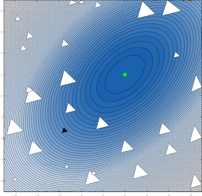
For my diploma thesis I needed an easy-to-use optimisation algorithm which could minimise a given function. I had access to Matlab, but surprisingly, none of the supplied optimisation functions seemed to satisfy my needs: I wanted to globally minimise a non-linear function within boundaries without using gradients.
So I did a little research and found a Globalized Nelder-Mead method (PDF), which is a tuned version of the good old downhill simplex algorithm. Then I implemented it as a Matlab function. By the way: the function also works fine with Octave.
What does it do?
The Nelder-Mead algorithm, sometimes also called downhill simplex method, was originally published in 1965. It is an iterative algorithm for local, unconstrained minimisation of a non-linear function $latex f : \mathbb{R}^n \to \mathbb{R}$. In contrast to most other iterative algorithms, it does not rely on the derivative of the target function but only evaluates the function itself. This makes it extremely well suited for cases when the target function is not an algebraic term, but a simulation model which cannot be derived directly. It also does not approximate the function’s gradient but is based on geometrical projections of an n+1-point polygon—the simplex—in the n-dimensional parameter space of the target function. A simplex in two dimensions is a triangle, one in three dimensions is a tetrahedron. In general, the simplex can be represented as a matrix $latex \mathbf{S} \in \mathbb{R}^{(n)\times(n+1)}$ of its points:
$latex \mathbf{S} = \begin{bmatrix} \mathbf{x}_0 & \cdots& \mathbf{x}_n \end{bmatrix} \text{ with } \mathbf{x}_i \in \mathbb{R}^n$
The basic idea behind the simplex algorithm is that the worst point of $latex \mathbf{S}$ is replaced by a better one with a smaller function value and to repeat this operation iteratively until a local optimum has been found. To achieve this, three different transformations are applied to the simplex which let it move in directions of descent and shrink around a local minimum. These transformations are called reflection, expansion and contraction.
In each iteration, first the worst point is reflected at the centroid of the remaining points. Depending on the quality (good or bad) it then replaces the worst point in the simplex. If the reflected point is not better, it is withdrawn and the other fallback operations are executed.
The globalized Nelder-Mead method just generalizes this idea to find a global minimum. Instead of initialising the simplex once, multiple simplices are initialised and each one finds one local minimum. There are some tweaks to make the location of these simplices better than random, but principally they are spread randomly within the allowed boundaries.
How do I use it?
Just copy the file gbnm.m from the download below into a directory where Matlab or Octave can find it. Then just call the function gbnm. A typical usage might look like this:
[code lang=”matlab”]
% Define test function and optimisation boundaries
f = @(x) norm(x).^2 – cos(norm(x));
xmin = [-10;-10];
xmax = -xmin;
xoptim = gbnm(f,xmin,xmax)
% Expected output: xoptim = [0.00.. ; 0.00..]
[/code]
The function does not only return the found minimum and has an optional argument for tweaking the algorithm parameters:
[code lang=”matlab” light=”true”]
[x, fval, output, options] = gbnm(fun,xmin,xmax[, options])
[/code]
Refer to the output of help gbnm and the research paper for further detail. If something remains unclear or you have found a bug, feel free to comment or post an issue on GitHub!
Download
The source has been moved to GitHub: repository ojdo/gbnm contains the function file, and a proper README file.
Original release (deprecated):
gbnm.zip (v0.1 [2010-07-19] initial release)


Comments
8 responses to “Optimise nonlinear functions using Matlab or Octave”
Hello
I put the example in Matlab, but each run, the gbnm function gives me different results, for instance different x and fval.
Have a good night,
Chris
The example run should (nearly) always return the same values. Small numerical differences are to be expected, but the example I posted should always find a point pretty close to
[0;0]as optimal. Can you post the exact function and values for xmin and xmax you used?Yes, you are right. I use the banana function
ff=inline('100*(x(2)-x(1)^2)^2+(1-x(1))^2','x');the results from each run are almost the same.
Thank you very much for this wonderful function,
Chris
Sehr gut, sehr gut! 🙂
Ich hatte in meiner Projektarbeit auch mit (nichtlinearer) Optimierung zu tun. Vielen Dank für den interessanten Artikel.
Beste Grüße aus Erlangen
Peter
Hi,
How should I use your gbnm function if my function to be optimized cannot be expressed in an analytical form? For example, my function is
function out=jinsong(phi)
where phi is a 9×9 array.
Many thanks for your help.
Jinsong
gbnmat the moment only can optimise functions that take a column vector as an input. But with a one-line wrapper function you can make your function compatible:jinsongv = @(phiv) jinsong(reshape(phiv,3,3))This function can be called with a 9 element column vector
phivand thus be handed to gbnm. Of course you have to reshape xmin and xmax the same way.Oh, and one remark: 9 variables is more than I ever have tried to use this algorithm for. If you get unsatisfying results, try reducing complexity by fixing some (k) of the 9 variables by setting xmin(k) equal to xmax(k).
hi, i seem to be having the same problem as chris.
my values for xmin are:
[-1.20;-0.23;-0.94]xmax:
[1.00;1.26;1.97]and my function is
(1-x(1))^2+10*(x(2)-x(1)^2)^2Tebello: your function only uses `x(2)` and `x(1)`, yet your boundaries have three entries. What is `x(3)` for? And: what does not work for you? For me,
gbnmfinds point[1; 1; ...]to be optimal, where `x(3)` can be any value because it does not occur in the function.[code]
octave:1> xmin = [-1.20;-0.23;-0.94];
octave:2> xmax = [1.00;1.26;1.97];
octave:3> f = @(x) (1-x(1))^2+10*(x(2)-x(1)^2)^2;
octave:4> gbnm(f, xmin, xmax)
ans =
1.00000
1.00001
-0.57791
[/code]